8 Power

In most experiments, our goal is to estimate the effect of one or more treatments—either by testing whether the treatment effects are zero or by obtaining confidence intervals for their sizes. Before we conduct an experiment, then, we must ask: How many experimental units do we require?

This question can be phrased in two ways:

How many experimental units do we need to reject the null hypothesis of no treatment effect with high probability, provided there really is a treatment effect?
How many experimental units do we need to estimate the treatment effect with a confidence interval of a desired width?

Strangely, neither of these questions is emphasized much in classic experimental design theory, perhaps because industrial and agricultural experiments are already subject to many constraints limiting their sample size. If you can only afford a certain number of trials, or only have so many plots of land, you design the experiment to use them all.

Also, industrial experiments are typically designed to minimize the error variance \(\sigma^2\). If a chemical refining process is highly repeatable, so that running it with the same input settings will produce a very similar response, then the input settings can be manipulated without worrying too much about the effect of random variation. Or, in short, if \(\sigma^2\) is very small, most observed effects will be real and any experiment will be powerful.

It is only in other settings, such as clinical trials or experiments on website users, where the experimenter may have the ability to choose the sample size target. These settings also have a great deal of error variance: every patient in a clinical trial will likely have a different response to the treatment, and the behavior of users on websites is very random. Here \(\sigma^2\) is large and the experimenter must obtain a sample size large enough to average out the variation.

When sample size is discussed, it’s mainly focused on the first question, the question of statistical power for null hypothesis tests. However, the second question is more important. Confidence intervals are more useful than hypothesis tests in general; failing to reject a null hypothesis is much more informative when you know the precision of the estimate.

Nonetheless, let’s consider the first question first.

8.1 Power of tests

8.1.1 One-way experiments

Suppose your research question can be answered with a \(F\) test (Section 6.6.2). For instance, in a simple experiment with one treatment factor with three levels, you might be interested in the null hypothesis \[ H_0: \tau_1 = \tau_2 = \tau_3, \] reflecting all treatment means being the same. If treatment 1 is a control and treatments 2 and 3 are new treatments, this null represents the new treatments working no better than control.

An \(F\) test for this null would amount to fitting the model with the factor and the model with only an intercept, then calculating the \(F\) statistic to compare them. We previously worked out the distribution of \(F\) under \(H_0\), finding that it follows an \(F\) distribution with degrees of freedom depending on the sample size and number of treatments.

It turns out we can also obtain the \(F\) statistic’s distribution under an alternative hypothesis.

Theorem 8.1 (Alternative distribution for the partial F test) In a partial \(F\) test for a treatment factor with \(v\) levels, each with \(r_i\) replicates, the \(F\) statistic has distribution \[ F_{v-1, n-v, \delta^2}, \] where this represents the noncentral \(F\) distribution, and \[\begin{align*} \delta^2 &= \frac{(v - 1) Q(\tau)}{\sigma^2}\\ Q(\tau) &= \frac{\sum_{i=1}^v r_i \left(\tau_i - \frac{1}{n}\sum_{h=1}^v r_h \tau_h\right)^2}{v-1}. \end{align*}\] We can think of \(Q(\tau)\) as representing the variance of the treatment means. \(\delta^2\) is the noncentrality parameter, which defines the shape of the noncentral \(F\) distribution along with the two degree of freedom parameters.

We can use Theorem 8.1 to calculate the power of the \(F\) test under a particular alternative hypothesis. To do so, we calculate the critical value of the null \(F\) distribution. We then calculate the probability of obtaining an \(F\) statistic equal to or larger than the critical value under the alternative.

Example 8.1 (Power in a simple binary experiment) Consider a simple experiment with \(v = 2\) treatments, each replicated \(r = 4\) times. We can calculate the critical value of the \(F\) statistic under the null:

v <- 2 # treatments
r <- 4 # replicates
n <- r * v # total sample size
alpha <- 0.05 # desired alpha level

f_crit <- qf(1 - alpha, v - 1, n - v)
f_crit

[1] 5.987378

Now we consider the alternative hypothesis where \(\tau_2 - \tau_1 = 1\). We might choose this particular alternative because we believe a difference of 1, in whatever units the response is measured in, is the smallest meaningful or important difference; if the true difference is smaller, we don’t care about detecting it.

Now we find the probability of obtaining a value equal to or more extreme than this one under the alternative hypothesis, using the noncentral \(F\). To calculate this we need \(\delta^2\) and hence \(Q(\tau)\). We will also need a value for \(\sigma^2\); we’ll suppose that in this experiment, it’s reasonable to guess that \(\sigma^2 = 2\).

Because \(r_i = r = 4\) for all \(i\), the difference between \(\tau_i\) and its mean is \(1/2\) for all \(i\), so we calculate \(Q(\tau)\) and \(\delta^2\) as:

sigma2 <- 2
Q <- n * (1/2)**2 / (v - 1)
delta2 <- (v - 1) * Q / sigma2

To find the power, i.e., the probability of obtaining an \(F\) statistic larger than f_crit, we use pf with the ncp argument to set the noncentrality parameter:

power <- pf(f_crit, v - 1, n - v, ncp = delta2, lower.tail = FALSE)
power

[1] 0.1356114

Evidently we have only 14% power in this scenario. If we double the number of replicates, we get:

r <- 8
n <- r *  v
f_crit <- qf(1 - alpha, v - 1, n - v)
Q <- n * (1/2)**2 / (v - 1)
delta2 <- (v - 1) * Q / sigma2
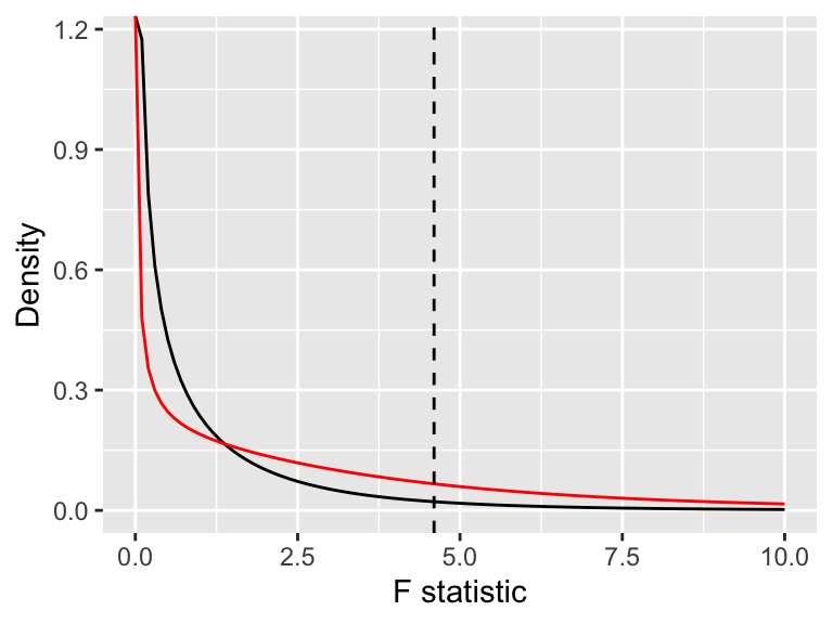
pf(f_crit, v - 1, n - v, ncp = delta2, lower.tail = FALSE)

[1] 0.2610284

We can also visualize the power in Figure 8.1. Here we’ve plotted the density of the null and alternative \(F\) distributions, along with the critical value. We can see that despite the null hypothesis being false, small \(F\) statistics still have high density. This experiment is underpowered.

Figure 8.1: \(F\) statistic distribution under the null hypothesis (black) and alternative hypothesis (red). The area under the black curve to the right of the dashed line is 5%; the same area under the red curve is the power.

Naturally, we can choose the necessary sample size for our experiment by setting a desired power level and then finding the \(r\) necessary to achieve that power. There is no uniform rule for the “right” power of an experiment. If you really care about whether a treatment effect exists, you should insist on a power near 100%; if you must conduct many experiments cheaply and are willing to accept missing true signals some of the time, you might accept lower power. The most commonly used power threshold is 80%, probably because it’s a nice round number that someone proposed early in the literature and everyone else copied.

Also, the procedure above requires us to specify the value of every \(\tau\) under the alternative. In a treatment with several levels, this is inconvenient. If I’m interested in testing whether any treatment is different from the others by a certain amount, do I need to consider every possible configuration of \(\tau\) that includes a difference of that amount?

Fortunately we can rearrange Theorem 8.1 to handle the worst-case alternative hypothesis.

Theorem 8.2 (Worse-case alternative distribution for the \(F\) test) Consider a one-way experiment with \(v\) levels. There are many possible alternative hypotheses where the largest difference between treatments is \(\Delta\): \[ \Delta = \max_{ij} |\tau_i - \tau_j|. \] When all treatments have \(r\) replicates, the alternative hypothesis with difference \(\Delta\) with lowest power is that in which

all but two treatments have the same mean
one treatment has mean \(\Delta/2\) lower
one treatment has mean \(\Delta/2\) higher.

In this worst case, we can use Theorem 8.1 with \[ \delta^2 = \frac{r \Delta^2}{2 \sigma^2} \] to calculate the power.

By calculating the power in the worst possible case, we know that in other alternatives with maximum difference \(\Delta\), the power would be higher. We can choose our sample size to attain power in the worst case and be confident of having at least that much power in any alternative we care about.

Theorem 8.2 also has an appealing benefit: it can be naturally parametrized in terms of \(\Delta/\sigma\), the size of the largest difference relative to the standard deviation of the errors. For instance, if \(\Delta/\sigma = 1\), we’re looking for a 1-standard-deviation difference.

Power calculations can be used in two different ways in practice:

In some experiments, the number of units is fixed by practical considerations. If we find the power is too low, we can reduce the number of treatments \(v\), allowing us to have more replicates in the remaining treatments.
If we do have the power to gather additional experimental units, we can increase \(r\) until we obtain the desired power.

8.1.2 More complex designs

Similar power calculations can easily be extended to designs where the desired hypothesis can be tested with an \(F\) test, and the factor of interest is orthogonal to the blocks or other treatment factors.

Recall that when the treatments and blocks are orthogonal to each other, we can fit the factors completely separately, rather than needing one model with all factors. (That was the major appeal of orthogonal designs pre-computers.) In other words, we can analyze a blocked or multifactor design as a one-way design, after we subtract out the other factors or blocks.

That subtraction does not change the mean estimates. It only affects how we estimate \(\hat \sigma^2\). Consequently, we can reuse the results of the previous subsection, substituting in the correct number of treatments for the test of interest and an estimate of \(\sigma^2\) after blocking and other orthogonal treatments have been accounted for.

Example 8.2 (Power in a factorial experiment) Consider a factorial experiment (Section 7.1) with two treatment factors, one with \(v_1 = 3\) levels and one with \(v_2 = 4\) levels. We’ll imagine we’re doing a full factorial design with \(r = 2\) replicates per cell, modeled without an interaction. This design is orthogonal.

Let’s use Theorem 8.2 to consider the power to detect an effect for treatment 1, in terms of the standardized effect size \(d = \Delta/\sigma\). For treatment 1, the critical value of the \(F\) test would be:

v <- 3
r <- 2
n <- r * v
alpha <- 0.05

f_crit <- qf(1 - alpha, v - 1, n - v)

This is identical to the calculation in Example 8.1. To calculate the power as a function of \(d\), let’s define a function that takes \(d\) as an argument and calculates the probability under the alternative noncentral \(F\):

worst_case_power <- function(d) {
  delta2 <- r * d^2 / 2

  return(pf(f_crit, v - 1, n - v, ncp = delta2, lower.tail = FALSE))
}

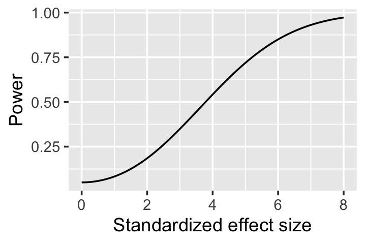
The resulting power curve is plotted in Figure 8.2 and illustrates that only relatively large effects can be reliably detected—those where the largest difference between treatments is several standard deviations. Again, this is relative to the variance \(\sigma^2\), which is the variance in the response conditional on treatment, rather than the marginal variance of the response.

Figure 8.2: Power of the experiment described in Example 8.2.

8.1.3 Contrasts

Besides \(F\) tests for treatment factors, we may also be interested in specific contrasts. If we fix a particular contrast vector \(c\) in advance of the experiment, we can use Theorem 6.1, Theorem 6.2, and their extension to multifactor experiments to conduct the test, and hence to derive the power of the test.

Theorem 6.2 defines the statistic \(T = \sum_i c_i \tau_i\) and its estimate \(\hat T\), and shows that for a null hypothesis \(H_0: T = t_0\), we can normalize \(\hat T\) by its estimated variance to obtain a test statistic with a \(t\) distribution. Consider a particular alternative hypothesis \(H_A: T = t_A\), where \(t_A \neq t_0\). Then the test statistic \[ \frac{\hat T - t_0}{\sqrt{\widehat{\var}(\hat T)}} \] will not have mean 0 and will not be \(t\)-distributed. Instead, it will follow the noncentral \(t\) distribution.

Theorem 8.3 (Distribution of contrasts under the alternative) Consider an experiment with \(r\) replicates per cell and a contrast vector \(c\), normalized so that \(\sum_i c_i^2 = 1\). When testing the contrast \(T = \sum_i c_i \tau_i\) under the null hypothesis \(H_0: T = t_0\), when the alternative \(H_A: T = t_A\) is true (and \(t_A \neq t_0\)), the test statistic is distributed as \[ \frac{\hat T - t_0}{\sqrt{\widehat{\var}(\hat T)}} \sim t_{n - v, \delta}, \] where \(\delta = \sqrt{r}(t_A - t_0)/\sigma\) is the noncentrality parameter of the noncentral \(t\) distribution.

Proof. By definition, a noncentral \(t\) distribution arises when we have a standard normal random variable \(Z\), a \(\chi^2\) random variable \(V\) with \(\nu\) degrees of freedom, and a scalar \(\mu\), and calculate \[ \frac{Z + \mu}{\sqrt{V / \nu}}. \] So we must rewrite test statistic in this form. We can start by trying to isolate a standard normal: \[ \frac{\hat T - t_0}{\sqrt{\widehat{\var}(\hat T)}} = \frac{\frac{\hat T - t_A}{\sqrt{\var(\hat T)}} + \frac{t_A - t_0}{\sqrt{\var(\hat T)}}}{\sqrt{\widehat{\var}(\hat T)} / \sqrt{\var(\hat T)}}. \] According to Theorem 6.1, when \(\sum_i c_i^2 = 1\) and \(r_i = r\), \[ \var(\hat T) = \frac{\sigma^2}{r}. \] Substituting this in, we obtain \[ \frac{\hat T - t_0}{\sqrt{\widehat{\var}(\hat T)}} = \frac{\frac{\hat T - t_A}{\sqrt{\sigma^2/r}} + \frac{t_A - t_0}{\sqrt{\sigma^2/r}}}{\sqrt{\widehat{\var}(\hat T)}/\sqrt{\sigma^2 / r}}. \] The numerator consists of a standard normal plus a constant, as desired. In the denominator, \(\widehat{\var}(\hat T) = \hat \sigma^2 / r\), where \(\hat \sigma^2 = \RSS / (n - v)\), so the denominator becomes \[ \sqrt{\frac{\frac{\RSS}{r(n - v)}}{\sigma^2 / r}} = \sqrt{\frac{\RSS/\sigma^2}{n-v}}. \] This is a \(\chi^2_{n-v}\) random variable divided by its degrees of freedom, so we have the desired result.

Example 8.3 (Equivalence of contrast and \(F\) test) Consider an experiment with \(v = 2\) treatments. We wish to test \(H_0: \tau_1 = \tau_2\) against the alternative \(H_A: \tau_2 - \tau_1 = \Delta\). We could use Theorem 8.2, in which case we would conduct an \(F\) test and use the noncentral \(F\) as the alternative distribution, with noncentrality parameter \[ \delta^2 = \frac{r \Delta^2}{2 \sigma^2}. \]

We could test the same hypothesis with the contrast vector \[ c = \begin{pmatrix} -\frac{1}{\sqrt{2}} \\ \frac{1}{\sqrt{2}} \end{pmatrix}, \] which is scaled to meet the requirement that \(\sum_i c_i^2 = 1\). Under the alternative \(H_A\), \[ T = \frac{\tau_2 - \tau_1}{\sqrt{2}}, \] so \(t_A = \Delta/\sqrt{2}\). Following Theorem 8.3, the noncentrality parameter is \[ \delta = \frac{\sqrt{r} (\Delta/\sqrt{2} - 0)}{\sigma} = \frac{\sqrt{r}\Delta}{\sqrt{2} \sigma}. \] It is not a coincidence that this is the square root of the \(F\) noncentrality parameter: in a case like this, the square of the \(t\) statistic is the same as the \(F\) statistic, and the square of the noncentral \(t\) is the noncentral \(F\).

8.1.4 Simulation

The analytical approaches to power above required certain simplifying conditions, such as an equal number of units \(r\) in each cell. The extension of \(F\) test power calculations to multifactor experiments also required those factors to be orthogonal. This limits the type of experiments we can calculate power for. Also, if we add covariates with ANCOVA (Section 6.7), none of the methods above will apply.

An alternative approach to calculate power is to simulate data from the experiment: draw the appropriate number of samples, run the desired analysis, calculate the test result, and repeat many times. The fraction of simulations that yield a significant result is the power.

Simulation has the advantage that it can be used for any alternative hypothesis that can be simulated, even if one can’t do the math to calculate the distribution under the alternative. If we have a design with non-orthogonal blocks, or expect the errors to be particularly non-normal, or have weird imbalances—it may not be easy to derive the distribution under the alternative, but we can certainly simulate it.

TODO example

8.2 Precision

Besides setting the sample size to obtain a particular statistical power, it is also reasonable to set it to obtain a particular precision. If we are interested in a particular contrast, we could ask: What sample size is necessary to make that contrast’s confidence interval sufficiently narrow? A wide CI gives us very little information about the contrast of interest, so we could specify in advance how narrow we would like it to be, then design our experiment to achieve that goal.

Based on Theorem 6.3, the width of a confidence interval for a contrast \(T = \sum_i c_i \tau_i\) is \[ 2 t_{n - v, 1 - \alpha/2} \sqrt{\widehat{\var}(\hat T)}. \] Now, \(\widehat{\var}(\hat T)\) depends on the sample, but we can use the population \(\var(\hat T)\) if we can guess \(\sigma^2\) in advance of the experiment. Then we can solve for the values of \(n\) and \(r\) required to obtain our desired confidence interval width.

This is not a guarantee, since the actual CIs will be calculated using \(\widehat{\var}(\hat T)\), which may be larger or smaller than the true \(\var(\hat T)\). In principle it is possible to calculate the distribution of \(\widehat{\var}(\hat T)\) and hence choose a sample size that will, for instance, produce confidence intervals narrower than a target width at least 80% of the time (Maxwell, Kelley, and Rausch 2008). In practice, I have never seen someone bother to do this in experimental design.

8.3 Exercises

Exercise 8.1 (Power of an F test) Consider an experiment with \(v = 4\) treatments. Suppose our alternative hypothesis is \[ H_A: \tau_1 = \tau_2 = \tau_3 = \tau_4 + 4, \] so one treatment group differs by 4. Based on a pilot study, we believe \(\sigma^2 \approx 8\).

Calculate the power of the test for different sample sizes, from \(r = 2\) to \(r = 10\), assuming \(\alpha = 0.05\). What \(r\) is necessary to achieve at least 80% power?