13 Observational Design

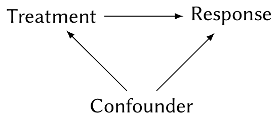
In Chapter 2, we discussed the standard reason to do an experiment. Suppose we want to know the effect of a treatment on a response, but there is a confounder:

By randomly assigning treatment, we can break the arrow from the confounding variable to treatment, thus allowing us to estimate the effect of treatment on response. To get the best possible estimate, we used all our experimental design techniques, such as blocking and control of covariates.

What if we can’t assign the treatment? We then have an observational study, so we are limited to measuring associations—but if we are willing to make some assumptions, and if we observe the relevant confounding variables, we may be able to get close to the causal effect.

Consider the case where the treatment is binary, so we can denote it as \(Z_i \in \{0, 1\}\). Let \(\pi_i = \Pr(Z_i = 1 \mid X_i = x_i)\) for each unit \(i\), where \(X_i\) are the covariates (including the confounders). In an experiment, \(\pi_i\) is under our control: we choose it based on our design, and it reflects the randomization procedure we select. Because we choose it, there is no arrow from confounder to treatment.

But in an observational study, \(\pi_i\) may depend on the confounder. It may be unknown: we do not know how the confounder affects the treatment, just that it does. How it varies matters. If \(\pi_i = 0.5\) for all \(i\), then the confounder has no effect on the treatment, and it is not a confounder at all—so we may safely conclude association is causation. If \(\pi_i\) is larger for people who will respond well to the treatment and smaller for people who won’t, then on average, the people who receive the treatment will also have a better response, and we will overestimate its effect.

Suppose, then, that we could estimate \(\pi_i\) and extract out everyone with a similar value of it. We could then take a subgroup for whom, say, \(\pi_i \approx 0.4\). Within this group, the confounder does not affect the treatment, and so we may estimate the association between treatment and response. We could repeat this for subgroups with \(\pi_i \approx 0.5\), \(\pi_i \approx 0.6\), and so on, and combine the results to form an estimate of the overall effect.

That suggests several possible strategies to estimate a causal effect, even in an observational study:

Attempt to model \(\pi_i\) and then group together units with similar values. Conduct analysis within each group. This is a stratified analysis.
Match up units with \(Z_i = 0\) and \(Z_i = 1\) that have similar values of \(\pi_i\). Compare each treated unit to its companion control unit. This is called matching.
Build a model to estimate \(\pi_i\) and use the predicted values in your model as a control variable.

Each of these has its uses. Let’s start with the foundations.

13.1 Propensity scores

Let’s redefine \(\pi_i\) as a propensity score. In general, the probability of treatment may depend on both observed covariates and unobserved covariates, and perhaps even the potential outcomes \(C_i(Z_i)\), so let’s include all of those.

Definition 13.1 (Propensity score) In an observational study with treatment \(Z_i\), observed covariates \(X_i\), unobserved covariates \(U_i\), and potential outcomes \(C_i\), the propensity scores are the values \[ \pi_i = \Pr(Z_i = 1 \mid X_i = x_i, Z_i = z_i, C_i(0), C_i(1)). \] We interpret them as the propensity to receive the treatment (\(Z_i = 1\)) given all the factors that may influence it.

We can think of the propensity scores as summarizing all the information (contained in the covariates) relevant to whether or not you receive the treatment. TODO show concretely that these are sufficient to estimate the causal effect from the observed data

Suppose the observed covariates \(X_i\) are the only things that affect the probability of treatment—there are no unobserved confounders. In this situation, we say the treatment assignment is “strongly ignorable” given \(X\).

Definition 13.2 (Strong ignorability) If the propensity score (Definition 13.1) can be written as \[ \pi_i = \Pr(Z_i = 1 \mid X_i = x_i), \] without unobserved confounders or potential outcomes, if \(0 < \pi_i < 1\) for all \(i\), and if the treatment assignments are conditionally independent given \(X\), we can say the treatment assignment is strongly ignorable given the observed covariates \(X\).

As we will see below, if the treatment assignments are strongly ignorable, we can simply perform matching: match up two units with \(Z_i = 0\) and \(Z_i = 1\) whose values of \(X\) are nearly identical. Their difference in response should estimate the causal effect.

We can’t test strong ignorability from the observed data, as we can’t test the association between \(Z_i\) and unobserved data without observing it. Judging whether it holds depends on your understanding of the assignment mechanism.

Regardless of whether the strong ignorability assumption holds, the propensity score based on the observed covariates summarizes all the information about them that is relevant to assignment.

Theorem 13.1 (Balancing property) The treatment and covariates are conditionally independent given the propensity score: \[ Z_i \perp X_i \mid \lambda(x_i), \] where \(\lambda(x)\) is the propensity score function on the observed covariates: \[ \lambda(x) = \Pr(Z = 1 \mid X = x). \]

Proof. The independence means that \[ \Pr(X = x \mid \lambda(x) = \lambda, Z = 1) = \Pr(X = x \mid \lambda(x) = \lambda, Z = 0). \] We can show this is true with Bayes’ theorem: \[\begin{align*} \Pr(X = x \mid \lambda(x) = \lambda, Z = 0) &= \frac{\Pr(Z = 1 \mid \lambda(x) = \lambda, X = x) \Pr(X = x \mid \lambda(x) = \lambda)}{\Pr(Z = 1 \mid \lambda(x) = \lambda)}\\ &= \frac{\lambda \Pr(X = x \mid \lambda(x) = \lambda)}{\lambda}\\ &= \Pr(X = x \mid \lambda(x) = \lambda). \end{align*}\] So the distribution of \(X\) is independent of \(Z\), conditional on \(\lambda(x)\).

13.2 Matching

To estimate the causal effect despite confounders, our first intuition may be to condition on the confounders. That could be with a model, but a simpler approach is to group units with similar values.

TODO