10 Early Stopping

So far, we have considered experiments where we choose $n$, the number of experimental units, and then run the experiment. We obtain all $n$ results in one batch and proceed to the analysis.

But many experiments don’t work this way. In most, the data is collected over time, and results appear gradually as trials are completed. For example, in a clinical trial of a medication, we do not recruit all the patients on the same day. Instead, the study begins enrolling patients on a particular day, and then accepts new patients who appear over months or years; some patients will be done with the treatment long before other patients even enroll.

This is practical, because there may not be $n$ patients with the particular condition you’re studying all present at the hospital on the same day. You might only accumulate $n$ cases over several years. It spreads out the work and ensures your medical staff aren’t trying to treat $n$ people simultaneously.

But it also creates temptation. Can’t we peek at the early data to see how the experiment is going? If we’re lucky, we’ll have clear results long before we have all $n$ experimental units.

Similarly, if I’m running a trial of two versions of a website, new users appear gradually at their own pace. I can assign each new user to a treatment as they appear, and I will gradually get the sample size I need for my experiment.

In either case, there are good reasons to want to peek at the results early:

Each observation may be expensive. My experimental medical treatment might cost hundreds of thousands of dollars per dose, so if I can stop the trial early, I save lots of money.
Time is money. If I can stop early, I can move on to a new experiment sooner.
If the early results are strong, it may not be ethical to continue the experiment: If my new experimental treatment cures 100% of patients, and the old standard treatment only cures 50% of patients, then once I’m sure the new treatment works, I should give it to everyone. It seems cruel to keep assigning patients to the old treatment because my design says I need to. And if I’m trying two versions of a website, and one clearly makes more money than the other, there may be a good business reason to stop early and use the more profitable one.

That suggests a simple procedure: As soon as there is enough data to conduct the desired analysis (i.e. there’s at least one observation per treatment group and block, and so on), run the analysis. If the results are inconclusive, continue the study. If the results show the desired effect, stop the experiment. But this procedure has some problems.

10.1 Double-dipping

Consider the simplest possible early stopping procedure, which we might call a “sequential Bernoulli experiment”. In this experiment, experimental units arrive one at a time, and are randomly assigned to either treatment or control. The assignments are independent. Each unit’s response is measured immediately. We hence have a sequence $Z_1, Z_2, \dots$ of treatment assignments and a parallel sequence $Y_1, Y_2, \dots$ of response values. We assume that each treatment group has a separate mean, so that \[ \E[Y_i \mid Z_i = z_i] = \begin{cases} \mu_0 & \text{if $z_i = 0$} \\ \mu_1 & \text{if $z_i = 1$.} \end{cases} \] After each trial, we would like to conduct a test for the null hypothesis $H_0: \mu_0 = \mu_1$.

If the sample size were fixed, there are many tests we could use, the most obvious being a simple $t$ test for the difference in means. What if we simply use $t$ tests after every observation? For instance, after 10 observations we could conduct the test using $Y_1, \dots, Y_{10}$; then, after a further observation, conduct the test again using $Y_1, \dots, Y_{11}$. Repeat until we obtain a statistically significant result or reach our maximum budget for the experiment.

However, this procedure has a problem. Conducting multiple tests means a higher risk of false positives, as in any multiple-testing problem. Furthermore, each subsequent test’s results are correlated with all the previous tests, since the test after $t$ observations shares $t-1$ observations with the previous test. This makes the multiple testing difficult to exactly correct for, and without correction, we can obtain a significant result simply by waiting long enough and conducting enough trials, even when the null is true.

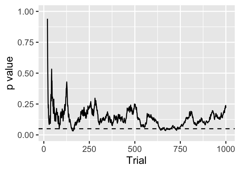
Example 10.1 (A sequential experiment with a true null) Let’s simulate an experiment where the null hypothesis is true. We’ll draw $Y$ from a standard normal distribution regardless of treatment assignment, and assign treatment independently at random. We will then conduct $t$ tests after each observation:

set.seed(2)

n <- 1000
fake_data <- data.frame(
  Y = rnorm(n),
  Z = rbinom(n, size = 1, prob = 0.5)
)

results <- data.frame(
  count = 20:n,
  p = NA
)

for (row in seq_len(nrow(results))) {
  count <- results$count[row]
  results$p[row] <- t.test(Y ~ Z, data = fake_data[1:count, ])$p.value
}

The sequence of $p$ values is shown in Figure 10.1. On average, the $p$ values should be $\operatorname{Uniform}(0, 1)$, as the null hypothesis is true, but it’s clear they are serially dependent. In this case there are several occasions when $p < 0.05$, so there are several opportunities for us to falsely declare a significant result.

Figure 10.1: The random walk of $p$ values for a sequential experiment where $t$ tests are conducted after every observation.

10.2 Sequential designs

Evidently we need test procedures that account for the sequential nature of the testing. One option comes from likelihood ratio tests.

Definition 10.1 (Likelihood ratio test) Consider obtaining samples $X_1, \dots, X_n \sim f$, where $f$ is a distribution parameterized by $\theta$. We would like to test $H_0: \theta \in \Theta_0$ against the alternative $H_A: \theta \in \Theta_0^c$. The likelihood ratio test statistic is \[ \lambda(X) = \frac{\sup_{\Theta_0} L(\theta \mid X_1, \dots X_n)}{\sup_\Theta L(\theta \mid X_1, \dots X_n)}, \] where $L(\theta \mid X_1, \dots, X_n)$ is the likelihood for $f$ given the parameters and data.

The likelihood ratio test has a rejection region of the form $\{X : \lambda(X) \leq c\}$, where $0 \leq c \leq 1$. Generally $c$ is chosen to obtain the desired $\alpha$-level.

You’ve likely used likelihood ratio tests before in your mathematical statistics courses. We can apply them to simple experimental sittings.

Example 10.2 (Likelihood ratio tests in experiments) Consider a trial with two treatment groups, denoted by $X_i \in \{0, 1\}$. We observe $Y$ and wish to test whether its mean is different between the two groups.

We can model \[ Y \sim \begin{cases} \text{Normal}(\mu_0, \sigma^2) & X_i = 0\\ \text{Normal}(\mu_1, \sigma^2) & X_i = 1 \end{cases} \] The parameter vector for the LRT is hence $\theta = (\mu_0, \mu_1)$. The null hypothesis is $H_0: \theta \in \Theta_0$, where $\Theta_0 = \{(\mu_0, \mu_1) : \mu_0 = \mu_1\}$.

Likelihood ratio tests have all kinds of desirable properties, which you undoubtedly explored in your mathematical statistics courses. They lead to two possible decisions: reject $H_0$ or fail to reject $H_0$.

We can extend likelihood ratio tests to produce sequential likelihood ratio tests. These allow three possible decisions: reject $H_0$, collect more data, or fail to reject $H_0$.

Definition 10.2 (Sequential likelihood ratio test) Consider obtaining a sequence of samples $X_1, X_2, \dots, X_n \sim f_n$, where $f_n$ is a joint distribution. We would like to test $H_0: f_n = f_{0n}$, for all $n$, against the alternative $H_A: f_n = f_{An}$ for all $n$. The likelihood ratio statistic is \[ \lambda(X) = \frac{f_{An}(X_1, \dots, X_n)}{f_{0n}(X_1, \dots, X_n)}, \] the ratio of densities/likelihoods.

We choose constants $0 < A < B < \infty$. At each $n$, our decision is \[ \text{decision} = \begin{cases} \text{reject $H_0$} & \lambda(X) \geq B\\ \text{obtain new sample} & A < \lambda(X) < B\\ \text{fail to reject $H_0$} & \lambda(X) \leq A \end{cases} \] We hence increase $n$ until we either reject or fail to reject. Denote the final sample size $N$.

(Siegmund 1985, sec. 2.1)

This test was first derived by Wald in the 1940s, and allows us to conduct the test after every observation. Each time, we either reject, fail to reject, or proceed to collect the next sample. The trick is determining the appropriate rejection region by setting $A$ and $B$; this involves some involved math, but can be directly calculated for some cases (Siegmund 1985, sec. 2.2). You can imagine conducting a more complicated version of this where the observations come from a designed experiment.

This test has some nice properties. Consider $\E_A[N]$, the expected final sample size under the alternative hypothesis, and $\E_0[N]$, the expected final sample size under the null. One can show that this test minimizes these sample sizes among all other sequential tests with the same size and power, although “a complete proof is circuitous and difficult” (Siegmund 1985, 9).

Sequential designs hence get use in certain niche applications where we can continuously analyze the data and immediately terminate the experiment. But they are not practical for many experiments:

We may not get all the data immediately after each unit is enrolled in the study. In a clinical trial, it may take months before we find out if the patient was cured; must we wait months between enrolling each patient?
We may not be able to easily run the analysis after each observation. Perhaps it is computationally intensive, or perhaps we are running a double-blind clinical trial out of many hospitals, and so we (the leaders of the study) do not receive data labeled with the treatment immediately.
It may not be possible to stop the trial at literally any time.

Consequently, it’s more common to design sequential experiments that let us enroll batches of experimental units. We enroll a batch, wait for their results, and then analyze the data to determine if more batches are necessary. Such a design is called a group sequential design.

10.3 Group sequential designs

Group sequential designs allow groups of experimental units to be enrolled in the study. As their results arrive, we can test for the presence of a treatment effect, and terminate the experiment early if we detect an effect.

Group sequential designs have become popular since the 1980s for clinical trials of new medications and surgeries, as they’re well-suited to the practical restrictions of large clinical trials. Large trials often have binary treatments (new treatment vs. old treatment or placebo) and enroll patients as they are found. Complicated blocking strategies are not used because they would require having all patients at the beginning of the study, so we could define the blocks and allocate treatments accordingly; simple block designs are often used, but require special care, as the experimenter may know how many patients have been allocated to each treatment and block so far, and hence know the treatment the next patient in a block will receive, breaking blinding. (TODO is this an accurate depiction of trial design?)

Consequently, most sequential design literature is on simple binary experiments without blocking and other fancy features.

For simplicity, let’s first consider a one-sample problem: We have a sequence of observations $X_1, X_2, \dots$ from a distribution with unknown mean $\mu$ and wish to test \[ H_0: \mu = \mu_0. \] How do we conduct such a hypothesis test in a group sequential fashion?

10.3.1 Setting critical values

In a group sequential design, we choose in advance $K$, the maximum number of groups to enroll. Each group has size $n_1, n_2, \dots, n_K$, so the maximum sample size is $N = \sum_{k=1}^K n_k$.

Following Wassmer and Brannath (2016), section 1.2, let’s index the observations by group. We observe, in sequence, \[ \underbrace{X_{11}, \dots, X_{1n_1}}_\text{group 1}, \underbrace{X_{21}, \dots, X_{2n_2}}_\text{group 2}, \dots, \underbrace{X_{K1}, \dots, X_{K n_K}}_\text{group $K$}. \] After each group of units is observed, we can calculate its group mean, \[ \bar X_k = \frac{1}{k} = \sum_{i=1}^{n_k} X_{ki}, \] and we can calculate the cumulative mean of all observations up to this stage: \[ \bar X^{(k)} = \frac{1}{\sum_{j=1}^k n_j} \sum_{j=1}^k n_j \bar X_j. \]

Now we need a test statistic. To test $H_0: \mu = \mu_0$, it seems reasonable to use a $z$ test, so we can define the $z$ statistic after group $k$ as \[ Z_k^* = \frac{\bar X^{(k)} - \mu_0}{\sigma} \sqrt{\sum_{j=1}^k n_j}, \] which would be standard normal when the data is normally distributed with known variance $\sigma^2$.

We could then define a rejection region for each test statistic $Z_k^*$. We would collect group 1, run the test for $Z_1^*$, and either stop (if significant) or continue (if not); if we continue, we’d collect group 2, run the test for $Z_2^*, and again either stop or continue. The process would repeat until group $K$.

However, defining the rejection region is not easy. The statistics $Z_1^*, \dots, Z_K^*$ are dependent, as they involve means of overlapping sets of random variables. The family-wise error rate, as defined in Section 6.6.3, is \[ \Pr(\cup_{k=1}^K \text{reject $Z_k^*$} \mid H_0), \] i.e. the probability that we reject any of the nulls under the alternative. The events are dependent. In principle we can still calculate this probability, as we can calculate the covariance between $Z_i^*$ and $Z_j^*$ and then work out the probabilities of each rejection; but even in the case where they are jointly multivariate normal, this begins to involve unpleasant integrals. It is difficult to work backwards and set the rejection region to attain a desired error rate $\alpha$.

10.3.2 Equally-sized groups

The problem becomes simpler—at least in terms of notation and algebra—when we define the groups to have equal size. This seems perfectly reasonable, and any logistical constraints limiting you to a particular size are likely to apply to every group.

When the groups are equally sized with $n = n_1 = \dots = n_K$, we can simplify the test statistic: \[ Z_k^* = \frac{1}{\sqrt{k}} \sum_{j=1}^k Z_k, \] where \[ Z_k = \frac{\bar X_k - \mu_0}{\sigma} \sqrt{n} \] is the test statistic for group $k$ alone. From this, one can derive that for $j \leq k$, \[ \cov(Z_j^*, Z_k^*) = \sqrt{\frac{j}{k}}, \] permitting easier calculation of the critical values. As $Z_k$ is based on sample averages, the sequence of test statistics is asymptotically multivariate normal with covariances given by this expression.

Probability calculations involving the tests, such as the probability of rejecting under the null, amount to manipulation of the multivariate normal. There are two common approaches to set rejection regions:

Set a rejection region that is the same for every $Z_k^*$, adjusting appropriately for their correlation and multiplicity.
Set rejection regions that monotonically shrink proportional to $\sqrt{k}$, again chosen appropriately for their correlation and multiplicity.

In either case, as the number of groups $K$ increases, the tests become more stringent (less powerful). See Wassmer and Brannath (2016), section 2.1, for details on exactly how to set the critical values.

10.3.3 Alpha-spending

TODO Wassmer and Brannath (2016), section 3.3

Group sequential designs are useful when we can easily fix the size of the groups in advance. However, in some experiments that may not be practical. In a clinical trial, for instance, patients are recruited over time, and we cannot easily predict how many patients will enroll at any particular time. Rather than budgeting for a fixed number of patients, we may budget to run the trial for a particular length of time; then it makes sense to check on the study at fixed time points, rather than at fixed sample sizes. This results in groups of unequal (and random) sizes.

To control the $\alpha$ level of the sequence of tests, we can use the “$\alpha$-spending” function.

Definition 10.3 (α-spending function) An $\alpha$-spending function is a non-decreasing function $\alpha^*(t)$ such that $\alpha^*(0) = 0$ and $\alpha^*(1) = \alpha$, where $\alpha$ is the desired overall $\alpha$ level of the sequential test procedure.

We choose $\alpha^*(t)$ in advance of the experiment. The sequence of results is broken into $K$ stages, after each of which we conduct a test. Let $n_k$ be the number of observations in stage $k$ and $N$ be the total number of observations. Then we can define the information rate $t_k$ for trial $k$ as \[ t_k = \frac{1}{N} \sum_{j=1}^k n_j, \] essentially the fraction of overall observations in the stages up to and including $k$. We will need the information rate to conduct each test, so we must fix the maximum sample size $N$ in advance of the study, though we need not choose the number of stages $K$ in advance.

After stage 1, we conduct a hypothesis test and set its critical value so its $\alpha$ level is $\alpha^*(t_1)$. We have now “spent” this portion of our overall $\alpha$ level. If the test is significant, we can stop the trial, knowing we have rejected the null with a test with a level smaller than $\alpha$; if the test is not significant, we continue to the next stage.

After stage 2, we conduct another hypothesis test. We set its critical value so that the probability of rejecting, conditional on the null and on not rejecting the first test, is \[ \Pr(\text{reject at stage 2} \mid H_0, \text{don't reject at stage 1}) = \alpha^*(t_2) - \alpha^*(t_1). \] In general it may be difficult to calculate the appropriate critical value; for the specific case of $z$ tests, the test statistics are multivariate normal and we can work out the dependence, so it is possible to use numerical integration to work out the appropriate critical value. We have now “spent” an additional increment of $\alpha$ level; adding up stage 1 and stage 2, we have spent a total of $\alpha^*(t_2)$.

The procedure repeats at each stage, setting the critical value at stage $k$ so that \[ \Pr(\text{reject at stage $k$} \mid H_0, \text{don't reject at previous stages}) = \alpha^*(t_k) - \alpha^*(t_{k-1}). \] If none are significant, this procedure repeats until we have experimented on all $N$ total units and the final information rate is $t_K = 1$. Summing up the critical values of each test, we find we have spent a total of $\alpha$, thus controlling the procedure to have the desired overall $\alpha$ level.

Clearly the choice of $\alpha^*(t)$ is important. If it rises quickly from 0, early tests will spend much of the overall $\alpha$, meaning less is left for later tests; in this case, the experiment is more likely to reject early, but later tests are more stringent. If it rises slowly from 0, early tests are stringent and less powerful, while later tests are more powerful. We can identify other desirable properties of the function:

$\alpha^*(t)$ should be monotone increasing. If it decreases from time $t_1$ to $t_2$, the required $\alpha$ level for the test at time $t_2$ would be negative, which is impossible.
$\alpha^*(t)$ should be continuous in $t$. If it has a jump discontinuity of size $\alpha^*$ at time $t^*$, and we conduct one test immediately before $t^*$ and one immediately after, then any test immediately afterward would have to have level at least $\alpha^*$, regardless of how soon it occurred after the previous test. This seems silly.

But there are many possible functions meeting these requirements.

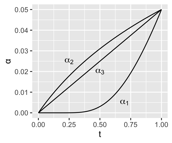
Example 10.3 (Common α-spending functions) Common $\alpha$-spending functions include: \[\begin{align*} \alpha_1^*(t) &= 4(1 - \Phi(\Phi^{-1}(1 - \alpha/4) / \sqrt{t})) \\ \alpha_2^*(t) &= \alpha \log(1 + (e - 1) t) \\ \alpha_3^*(\rho, t) &= \alpha t^\rho, \end{align*}\] where $\Phi$ is the standard normal cdf and $\rho$ is a positive tuning parameter. These functions are derived from prior group sequential procedures; for example, $\alpha_1^*$ is approximately the same as the group sequential procedure developed by O’Brien and Fleming (1979). It also seems to be the most commonly used $\alpha$ spending function.

Figure 10.2: Three choices of $\alpha$-spending functions. Here $\alpha_3^*$ is shown with $\rho = 1$.

In principle, it is possible to derive the power and expected sample size for various spending functions under different alternative hypotheses, and hence select an “optimal” function for the situation at hand. In practice, it seems large clinical trials select their $\alpha$ spending function while also choosing how many interim tests to conduct and at what times, then specify the desired power and $\alpha$ level at each time point based on clinical and ethical considerations. A spending function is then chosen to best suit these requirements. See the gsDesign package for a variety of tools for designing group sequential trials in this way.

10.3.4 Stopping for futility

It is also possible to design a sequential experiment that can stop the experiment if it is futile. If we are testing a one-sided hypothesis, such as “the treatment is better than the control”, we may want to stop the experiment if the treatment does spectacularly well in the first few groups—but we may also want to stop if it does poorly in the first few groups, as this would suggest we will not find evidence in favor of our alternative. Collecting further data would hence be futile.

This is again widely used in clinical trials, as we’d like to stop early if the treatment is not working or is even actively harming the patients.

It is possible to define futility stopping rules and adjust the test critical regions accordingly, although again, the math is tedious because of the correlation between the test statistics for each group.

10.4 Exercises

TODO